Introduction
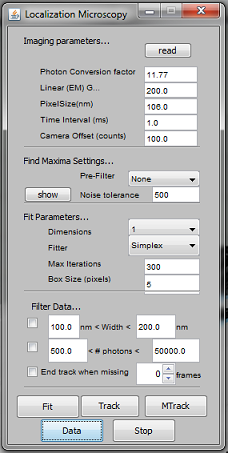
This plugin uses Gaussian fitting to localize single fluorescent molecules for tracking or reconstruction of super-resolution images. One window is used to set parameters for fitting and tracking, the second window (which can be opened from the first using the ‘Data’ button) is used to perform operations (such as rendering, drift correction, etc.) on data-sets of fitting results.
Getting Started
|
|
To track a spot of interest in a time-series, draw a box around the spot and press the ‘Track’ button. After a short while, a row will appear in the Gaussian tracking data Window. Select the row and press Plot to visualize movement of the spot in the x direction. To obtain a super-resolution image, acquire images using a square ROI with a size that is a power of 2 (256x256 often works best). Acquire a large data series of your blinking molecules (use the show button to get a feel for the number of spots that can be detected in your data). Press Fit to find spots and fit Gaussians to them. After a while, a row will appear in the Gaussian tracking data Window. Selected the row. Make sure the drop-down box in the Localization Microscopy section is set to 8x. Press Render. |
</table>
## Localization Microscope Window (first window)
|
|
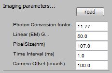
Imaging Parameters: |
</table>
|
|
Finding Maxima To find spots, the application searches the image using a box with the size given in the Fit Parameters section. The minimum difference (in digital numbers) between the center pixel and the average of the four corner pixels should be at least the value of the Noise tolerance field for a putative spot to qualify. The image can optionally be pre-filtered by obtaining the difference image of a Gaussian filter with a width equal to the pixel size and a Gaussian filter 5 times the pixel size. However, such pref-filtering rarely helps and will slow down calculations. The show button will show on the frontmost window what objects will be recognized as spots. |
</table>

|
|
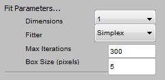
Fitting Parameters Dimensions: Determines the model used for the
Gaussian. 1 - results in symmetric Gaussian in which only the width can
vary, 2 - elliptical Gaussian, 3 - elliptical Gaussian in which the
angle (theta) of the blob can vary. See Wikipedia article on
Gaussian for details. |
</table>
|
|
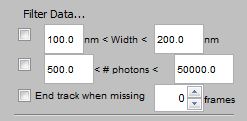
Filtering Data |
</table>
|
|
Data Processing |

|
|
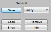
General Options Previously saved data can be loaded using the Load button. For text data to be recognized, they should resemble the text format saved by the application. TSF files can be opened, as well as the fitted data saved by the Nikon software. The Remove button will remove the selected row(s) from the table (saved data on disk will not be deleted). The Show button wil open a window with a table showing the fitted data (including the X, Y, and possibly Z location at each frame and channel, as well as information about spot width, and calculated number of photons detected). If the data set is large, it can take a long time for this window to open and it can take a large amount of RAM. The Info button will show some information about the data set (orginal image it was derived from, box size, original image size, pixel size, etc..). |
|
|
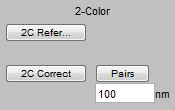
2-Color Single Molecule |
|
|
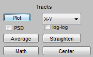
Processing Tracking Data |
|
|
Localization Microscopy |
