Camera characterization - Measuring the electron conversion factor, read-noise and offset using Photon Transfer Curves

–Nico 12:23, 30 September 2011 (PDT)

Based on a handout for the Bangalore Microscopy Course, 2011, modified for UCSF course BP210 March 2026.

Introduction

Figuring out which camera is best suited for your applications can be a daunting task. Luckily, most aspects of a camera can be described in straight forward physical terms and all scientific grade cameras should be delivered with a spec sheet detailing most aspects of the camera. However, it is also possible to determine some of these physical parameters yourself.

Parameters that strongly influence how well a camera performs under low light conditions are the readout noise and photon conversion factor. The readout noise is a constant amount of noise, mainly added by the CCD chip, readout amplifier and surrounding electronics. The faster the camera readout, the higher the readout noise. It is expressed in photo-electrons. The photon conversion factor relates the digital numbers associated with each pixel with the actual number of photo-electrons generated in each CCD (or CMOS) well. The photon-conversion factor changes when you change certain camera settings, such as the analogue and EM gain.

Below are methods to determine the camera’s readout noise and offset, approximate the electron conversion factor at different gain settings and fixed pattern noise. Please compare the numbers you find with the numbers on the data-sheet of the camera!

Constant/Even Illumination

To measure fixed pattern noise and the photon conversion factor, it is important to provide constant, even illumination. This is difficult to accomplish. One of the simplest ways is to use a smart phone with high resolution screen and display a white image (flashlight applications often have this capability). You can do this on a microscope by placing the phone flat on the microscope stage after switching to a low mag objective or removing the objective alltogether. If you have a camera that is not attached to a microsocpe, you can use a frosted disposable drinking cup (which is semi-transparent and scatters light a lot) over the entrance of the camera. Make sure that you have a light source that does not flicker at high frequencies (you can check this by collecting a time-lapse series at high frame rate / short exposure time and check for fluctuations in intenisty).

The best method to provide even illumination is by using an intergrating sphere.

Measuring Camera Characteristics

Visual inspection of fixed pattern noise in dark images

• Make sure no light reaches the camera (cap it, or direct the light path to another microscope port).
• In Micro-Manager, acquire a sequence of images by accessing the Multi-D Acquisition. Set the exposure time of the camera to 0 ms (or the minimum allowed by the camera), uncheck everything in the MDA window except for “Time points”, set the number of time points to 100 and the interval to 0 and press ‘Acquire”.
• Inspect the resulting data for irregularities. Does the average intensity stay constant:
  • First make a copy of the data into ImageJ by clicking the Gear icon and selecting “To ImageJ…”
  • Press control-A, in the ImageJ menu
  • Select “Analyze”->”Tools”->”ROI manager”
  • In the ROI manager press “Add”, then select “More” -> “Multi Measure”
  • Make sure “Measure all Slices” and “One row per slice” are checked and press OK)
  • To plot the data, copy the results table into a spreadsheet application.
• Calculate the sum using the ImageJ menu command ‘Image -> Stacks -> Z project…’. Choose the option ‘Sum of Slices’
• Inspect the resulting summed image for fixed patterns (look at the side, look for regular patterns).
• Repeat steps above using other readout speeds and/or gain (if available on your camera).
• Now set the exposure time to 1 second. Repeat the above (in the interest of time, reduce the number of exposuyres to 10). The noise you now may observe is called temporal read-noise and often show “hot pixels”.

Visual inspection for fixed pattern noise in bright images

• Use a smartphone (or preferably an integrating sphere) as illumination source (see introduction). Remove an objective from the microscope and place the phone on the microscope (it may even fit in the sample holder on the stage). Place it such that the image is as evenly illuminated as possible. Find an exposure time such that the maximum pixel value is about 90% of the highest value of the camera (you can use the Micro-Manager AutoExposure script for this purpose).
• Repeat steps listed above for dark images. You may note imperfections in the output image. Some imperfections are caused by uneven illumination and dust in the microscope or on the camera front window, the remainder is caused by fixed pattern noise in the camera. You can discriminate imperfections in your microscope from camera imperfections by rotating the camera 90 degrees and taking another data set (or rotate the camera while looking at a live image feed). Patterns that stay the same are caused by the camera, patterns that rotate 90 degrees are caused by your microscope.

Measure Offset and readout noise in digital numbers

Even when no light reaches the camera, there are variations in the measured pixel values caused by readout noise. Thus, if the average pixel value were to be zero, many pixels would have negative values. Negative values have no physical meaning and are hard to work with in a computer, therefore the camera manufacturers introduce an ‘offset’ (or, if they don’t, they should!) that sometimes can be changed by the end user. However, since you want to relate the digital numbers coming from your camera to a physical entity (the number of photons absorbed by a pixel), you will need to know what this offset is. Since the variation in pixel intensities of a ‘dark’ image is caused by readout noise, you can simply calculate the readout noise by calculating the standard deviation of the pixel intensity values in such a dark image. For a CMOS camera, the read-noise can differ from pixel to pixel, and it is better to acquire a stack of dark images and calculate the standard deviation per pixel.

• To measure the offset, take a single ‘dark’ image from the series described in 1 (or take a new one). Calculate the average intensity of the image or - if the camera has substantial fixed pattern noise - a subregion of the image (use the ImageJ command: Analyze->Measure). Make a note of the mean (which is the offset value expressed in digital numbers - DN).
• To measure the readout noise in digital numbers, take two ‘dark’ images (you can use ‘Snap’, then ImageJ menu, ‘Image’->’Duplicate’, then ‘Snap’ the second image). Subtract one image form the other (ImageJ menu: Process -> Image Calculator…, select the two images and subtract from each other). Open in a new window and use 32-bit (float) result. Calculate the standard deviation of the resulting image or a subregion if there are regions with detectable fixed pattern noise (ImageJ menu: Analyze->Set Measurements.. make sure that ‘standard deviation’ is checked, then select Analyze->Measure). The read-noise (in digital numbers) is the measured standard deviation divided by √2. The purpose of subtracting the two images is to remove fixed pattern noise. Make a note of the read-noise.

Estimate the electron conversion factor (electrons per digital number).

Theory: If a signal only contains Poisson (shot) noise, then:

σ(N)=√(N) with N = number of electrons

A camera generates images expressed in digital numbers (DN, sometimes called ADU: Analog-to-Digital Units) instead of electrons. The relation between digital numbers and electrons is given by:

N = c * DN

where c is the constant that we are interested in (the electron conversion factor). The following equation also holds true:

σ(N)=c . σ(DN)

Substituting the last two equations in the first and solving for ‘c’ yields:

c = DN/σ2(DN)

Thus, if imaging conditions can be established in which the only significant noise source is shot noise, then the relation between digital number and number of electrons can be determined without a need to know the absolute number of electrons striking the CCD!

To relate the signal and noise, one illuminates the camera with constant, even illumination, and then record images at varying intensities by changing the exposure time of the camera. From these images one calculates the (average) intensity and standard deviation (noise). Plotting noise against signal generates the Photon Transfer Curve.

The three main sources of noise are read-noise, shot noise, and fixed pattern noise. Read noise is a constant, shot noise scales with the square root of the signal, and fixed pattern noise scales with the signal. On a log-log plot, read noise will cause a slope of 0, shot noise causes a slope of 0.5, and fixed pattern noise causes a slope of

1. To find the area on the Photon Transfer Curve where shot noise is dominant, one needs to find the area where the slope is close to 0.5.



Photon Transfer Curve from: James R. Janesick, Photon Transfer, DN -> λ. SPIE Press, 2007

To facilitate measuring the photon conversion factor, we will remove fixed pattern noise by taking two images at each exposure time and calculate the noise after subtracting one image from the other.

• To create a Photon Transfer Curve and estimate the photon conversion factor and read-noise in electrons, we will use the Micro-Manager plugin “Photon Transfer Curve assistant” (Plugins > Acquisition Tools). This plugin fully automates taking stacks of images at increasing exposure times, calculating mean and standard deviation, plotting the data and calculating the electron conversion factor and read-noise.
• Provide uniform and constant illumination to the camera, then establish the maximum exposure time where you just start to see clipping of pixel intensities.

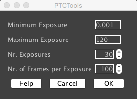
• Follow the instructions, you will end up with a plot with the Photon transfer curve, a table with the mean and standard deviation of each of the stacks, and a stack of images with the mean and standard deviation of each exposure. Inspect the latter for interesting patterns (which you may be able to see with CMOS cameras). Also take note of the highest value in the Photon Transfer Curve. Express that number in electrons, divide by the read-noise, and you have a measure for the dynamic range at these camera settings. You can also plot the exposure time against the mean to get an idea of the linearity of the camera response.

• Now change the gain (or EM gain if you have an EM CCD), and run the plugin again. This will change the electron conversion factor and possibly the read-noise.

References

For the complete theory behind photon transfer curves, consult the following reference: James R. Janesick, Photon Transfer, DN -> λ. SPIE Press, 2007.